
Quantum mechanics emerged in the beginning of the twentieth century as a new discipline because of the need to describe phenomena, which could not be explained using Newtonian mechanics or classical electromagnetic theory. These phenomena include the photoelectric effect, blackbody radiation and the rather complex radiation from an excited hydrogen gas. It is these and other experimental observations which led to the concepts of quantization of light into photons, the particle-wave duality, the de Broglie wavelength and the fundamental equation describing quantum mechanics, namely the Schrödinger equation. This section provides an introductory description of these concepts and a discussion of the energy levels of an infinite one-dimensional quantum well and those of the hydrogen atom. |
1.2.1 Particle-wave duality |   |
Quantum mechanics acknowledges the fact that particles exhibit wave properties. For instance, particles can produce interference patterns and can penetrate or "tunnel" through potential barriers. Neither of these effects can be explained using Newtonian mechanics. Photons on the other hand can behave as particles with well-defined energy. These observations blur the classical distinction between waves and particles. Two specific experiments demonstrate the particle-like behavior of light, namely the photoelectric effect and blackbody radiation. Both can only be explained by treating photons as discrete particles whose energy is proportional to the frequency of the light. The emission spectrum of an excited hydrogen gas demonstrates that electrons confined to an atom can only have discrete energies. Niels Bohr explained the emission spectrum by assuming that the wavelength of an electron wave is inversely proportional to the electron momentum. |
The particle and the wave picture are both simplified forms of the wave packet description, a localized wave consisting of a combination of plane waves with different wavelength. As the range of wavelength is compressed to a single value, the wave becomes a plane wave at a single frequency and yields the wave picture. As the range of wavelength is increased, the size of the wave packet is reduced, yielding a localized particle. |
1.2.2 The photo-electric effect | |
The photoelectric effect is by now the "classic" experiment, which demonstrates the quantized nature of light: when applying monochromatic light to a metal in vacuum one finds that electrons are released from the metal. This experiment confirms the notion that electrons are confined to the metal, but can escape when provided sufficient energy, for instance in the form of light. However, the surprising fact is that when illuminating with long wavelengths (typically larger than 400 nm) no electrons are emitted from the metal even if the light intensity is increased. On the other hand, one easily observes electron emission at ultra-violet wavelengths for which the number of electrons emitted does vary with the light intensity. A more detailed analysis reveals that the maximum kinetic energy of the emitted electrons varies linearly with the inverse of the wavelength, for wavelengths shorter than the maximum wavelength. |
The experimental setup is shown in Figure 1.2.1: |
 |
| Figure 1.2.1.: | Experimental set-up to measure the photoelectric effect. |
The experimental apparatus consists of two metal electrodes within a vacuum chamber. Light is incident on one of two electrodes to which an external voltage is applied. The external voltage is adjusted so that the current due to the photo-emitted electrons becomes zero. This voltage corresponds to the maximum kinetic energy, K.E., of the electrons in units of electron volt. That voltage is measured for different wavelengths and is plotted versus the inverse of the wavelength as shown in Figure 1.2.2. The resulting curve is a straight line. |
 |
| Figure 1.2.2 : | Maximum kinetic energy, K.E., of electrons emitted from a metal upon illumination with photon energy, Eph. The energy is plotted versus the inverse of the wavelength of the light. |
Albert Einstein explained this experiment by postulating that the energy of light is quantized. He assumed that light consists of individual particles called photons, so that the kinetic energy of the electrons, K.E= p2/2m equals the energy of the photons, Eph, minus the energy, qΦM, required to extract the electrons from the metal. The workfunction, ΦM,therefore quantifies the potential, which the electrons have to overcome to leave the metal. The slope of the curve was measured to be 1.24 eVμm, which yielded the following relation for the photon energy, Eph: |
 | (1.2.1) |
where h is Planck's constant, ν is the frequency of the light, c is the speed of light in vacuum and λ is the wavelength of the light. This relation between energy and frequency is identical to Max Planck’s assumption used to explain black body radiation, as described in section 1.2.3 |
While other light-related phenomena such as the interference of two coherent light beams demonstrate the wave characteristics of light, it is the photoelectric effect, which demonstrates the particle-like behavior of light. These experiments lead to the particle-wave duality concept, namely that particles observed in an appropriate environment behave as waves, while waves can also behave as particles. This concept applies to all waves and particles. For instance, coherent electron beams also yield interference patterns similar to those of light beams. |
It is the wave-like behavior of particles, which led to the de Broglie wavelength: since particles have wave-like properties, there is an associated wavelength, called the de Broglie wavelength and given by: |
 | (1.2.2) |
where λ is the wavelength, h is Planck's constant and p is the particle momentum. This expression enables a correct calculation of the ground energy of an electron in a hydrogen atom using the Bohr model described in Section 1.2.4. One can also show that equation (1.2.2) can be obtained by combining equation (1.2.1) with Eph = p c, which means that one combines the result from the photo-electric effect with the classical equation for particles, describing the kinetic energy by the product of its momentum and velocity.
|
Example 1.1  | A metal has a workfunction of 4.3 V. What is the minimum photon energy in Joule to emit an electron from this metal through the photo-electric effect? What are the photon frequency in Terahertz and the photon wavelength in micrometer? What is the corresponding photon momentum? What is the velocity of a free electron with the same momentum? |
| Solution | The minimum photon energy, Eph, equals the workfunction, ΦM, in units of electron volt or 4.3 eV. This also equals:
The corresponding photon frequency is:
The corresponding wavelength equals:
The photon momentum, p, is:
And the velocity, v, of an electron in vacuum with the same momentum equals
Where m0 is the free electron mass. |
1.2.3 Blackbody radiation | |
Another experiment which could not be explained without quantum mechanics is the blackbody radiation experiment: By heating an object to high temperatures one finds that it radiates energy in the form of infra-red, visible and ultra-violet light. The appearance is that of a red glow at temperatures around 800° C which becomes brighter at higher temperatures and eventually looks like white light. The spectrum of the radiation is continuous, which led scientists to initially believe that classical electromagnetic theory should apply. However, all attempts to describe this phenomenon failed until Max Planck developed the blackbody radiation theory. His theory is based on the assumption that the energy associated with light is quantized and that the energy quantum or photon energy equals: |
 | (1.2.3) |
Where ℏ is the reduced Planck's constant (= h/2π), and ω is the radial frequency (= 2π ν). |
The spectral density, uω, or the energy density per unit volume and per unit frequency is given by: |
 | (1.2.4) |
Where k is Boltzmann's constant and T is the temperature. The spectral density is shown versus energy in Figure 1.2.3. |
 |
| Figure 1.2.3: | Spectral density of a blackbody at 2000, 3000, 4000 and 5000 K versus energy. |
The peak value of the blackbody radiation per unit frequency occurs at 2.82 kT and increases with the third power of the temperature. Radiation from the sun closely fits that of a black body at 5800 K. |
| Example 1.2 | The spectral density of the sun peaks at a wavelength of 900 nm. If the sun behaves as a black body, what is the temperature of the sun? |
| Solution | A wavelength of 900 nm corresponds to a photon energy of:
Since the peak of the spectral density occurs at 2.82 kT, the corresponding temperature equals:
|
1.2.4 The Bohr model | |
The spectrum of electromagnetic radiation from an excited hydrogen gas was yet another experiment, which was difficult to explain since it is discrete rather than continuous. The wavelengths of the emitted photons were early on associated with a set of discrete electron energy levels En described by: |
 | (1.2.5) |
so that the emitted photon energies equal the energy difference released when an electron makes a transition from a higher energy Ei to a lower energy Ej. |
 | (1.2.6) |
The maximum photon energy emitted from a hydrogen atom equals 13.6 eV. This energy is also called one Rydberg or one atomic unit. The electron transitions and the resulting photon energies are further illustrated by Figure 1.2.4. |
 |
| Figure 1.2.4 : | Energy levels and possible electronic transitions in a hydrogen atom. Shown are the first six energy levels, as well as three possible transitions involving the lowest energy level (n = 1) |
However, at the time, there was no explanation why the possible energy values were not continuous. No classical theory based on Newtonian mechanics could provide such spectrum. Further more, there was no theory, which could explain these specific values. |
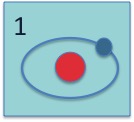
Niels Bohr provided a part of the puzzle. He assumed that electrons move along a circular trajectory around the proton like the earth around the sun, as shown in Figure 1.2.5. |
 |
| Figure 1.2.5: | Trajectory of an electron in a hydrogen atom as used in the Bohr model. |
He also assumed that electrons behave within the hydrogen atom as a wave rather than a particle. Therefore, the orbit-like electron trajectories around the proton are limited to those with a length equals to an integer number of wavelengths so that: |
 | (1.2.7) |
where r is the radius of the circular electron trajectory and n is a positive integer. The Bohr model also assumes that the momentum of the particle is linked to the de Broglie wavelength (equation (1.2.2)) |
The model further assumes a circular trajectory and that the centrifugal force equals the electrostatic force, or: |
 | (1.2.8) |
Solving for the radius of the trajectory one finds the Bohr radius, a0: |
 | (1.2.9) |
and the corresponding energy, En, is obtained by adding the kinetic energy, mv2/2, and the potential energy of the particle, V(r), yielding: |
 | (1.2.10) |
using as the potential energy,V(r), the electrostatic potential of the proton: |
 | (1.2.11) |
Note that all the possible energy values are negative. Electrons with positive energy are not bound to the proton and behave as free electrons. |
The Bohr model does provide the correct electron energies. However, it leaves many unanswered questions and, more importantly, it does not provide a general method to solve other problems of this type. The wave equation of electrons presented in the next section does provide a way to solve any quantum mechanical problem. |
1.2.5 Schrödinger's equation and selected solutions | |
A general procedure to solve quantum mechanical problems was proposed by Erwin Schrödinger. Starting from a classical description of the total energy, E, which equals the sum of the kinetic energy, K.E., and potential energy, V(x), or: |
 | (1.2.12) |
he converted this expression into a wave equation by defining a wavefunction, Ψ, and multiplied each term in the equation with that wavefunction: |
 | (1.2.13) |
To incorporate the de Broglie wavelength of the particle, we now introduce the operator, |
 | (1.2.14) |
Where k is the wavenumber, which equals 2π /λ. Without claiming that this is an actual proof, we now simply replace the momentum squared, p2, in equation (1.2.13) by this operator yielding the time-independent Schrödinger equation. |
 | (1.2.15) |
To illustrate the use of Schrödinger's equation, we present three solutions to Schrödinger's equation: that for an infinite quantum well, the hydrogen atom and tunneling through a barrier. Prior to that, we discuss the physical interpretation of the wavefunction. |
The use of a wavefunction to describe a particle, as in the Schrödinger equation, is consistent with the particle-wave duality concept. However, the physical meaning of the wavefunction does not naturally follow. Quantum theory postulates that the wavefunction, Ψ(x), multiplied with its complex conjugate, Ψ*(x), is proportional to the probability density function, P(x), associated with that particle. |
 | (1.2.16) |
This probability density function integrated over a specific volume provides the probability that the particle described by the wavefunction is within that volume. Therefore, the probability function must be normalized to indicate that the probability of finding the particle somewhere equals 100%. This normalization enables to calculate the magnitude of the wavefunction using: |
 | (1.2.17) |
This probability density function can then be used to find all properties of the particle by using the quantum operators. To find the expected value of a function f(x,p) for the particle described by the wavefunction, one calculates: |
 | (1.2.18) |
Where F(x) is the quantum operator associated with the function of interest. A list of quantum operators corresponding to a selection of common classical variables is provided in Table 1.2.1. |
 |
| Table 1.2.1: | Selected classical variables and the corresponding quantum operator. |
The one-dimensional infinite quantum well represents one of the simplest quantum mechanical structures. We use it here to illustrate some specific properties of quantum mechanical systems. The potential in an infinite well is zero between x = 0 and x = Lx and is infinite on either side of the well. The potential and the first five possible energy levels an electron can occupy are shown in Figure 1.2.6: |
 |
| Figure 1.2.6 : | Potential energy of an infinite well, with width Lx. Also indicated are the lowest five energy levels in the well. |
The energy levels in an infinite quantum well are calculated by solving Schrödinger's equation 1.2.15 with the potential, V(x), as shown in Figure 1.2.6. One therefore solves the following equation within the well: |
 | (1.2.19) |
The general solution to this differential equation is: |
 | (1.2.20) |
where the coefficients A and B must be determined by applying the boundary conditions. Since the potential is infinite on both sides of the well, the probability of finding an electron outside the well and at the well boundary equals zero. Therefore, the wave function must be zero on both sides of the infinite quantum well or: |
 | (1.2.21) |
These boundary conditions imply that the coefficient B must be zero and the argument of the sine function must equal a multiple of π at the edge of the quantum well or: |
 | (1.2.22) |
Where the subscript, n, was added to the energy, E,to indicate the energy corresponding to a specific value of, n. The resulting values of the energy, En, then equal: |
 | (1.2.23) |
The corresponding normalized wave functions, Ψn(x) are: |
 | (1.2.24) |
where the coefficient A was determined by requiring that the probability of finding the electron in the well equals unity or: |
 | (1.2.25) |
and Ψ*(x) is the complex conjugate of the wavefunction Ψ(x). |
Note that the lowest possible energy, namely E1, is not zero even though the potential is zero within the well. Only discrete energy values are obtained as eigenvalues of the Schrödinger equation. The energy difference between adjacent energy levels increases as the energy increases. An electron occupying one of the energy levels can have a positive or negative spin (s = ½ or s = -½). Both quantum numbers, n and s, are the only two quantum numbers needed to describe this system. |
The wavefunctions corresponding to each energy level are shown in Figure 1.2.7 (a). Each wavefunction has been shifted by the corresponding energy and scaled with an arbitrary magnitude as is commonly done. The probability density function, P(x)=Ψ(x)*Ψ(x), provides the probability of finding an electron at a certain location in the well. These (unnormalized) probability density functions are shown in Figure 1.2.7 (b) for the first five energy levels. For instance, for n = 2 the electron is least likely to be in the middle of the well and at the edges of the well. The electron is most likely to be one quarter of the well width away from either edge. |
 |
| Figure 1.2.7 : | (a) Energy levels, wavefunctions and (b) probability density functions in an infinite quantum well. The figure is calculated for a 10 nm wide well containing an electron with mass m0, the free electron mass. The wavefunctions and the probability density functions have an arbitrary magnitude (i.e. they are not normalized) and are shifted by the corresponding electron energy. |
| Example 1.3 | An electron is confined to a 1 micron thin layer of silicon. Assuming that the semiconductor can be adequately described by a one-dimensional quantum well with infinite walls, calculate the lowest possible energy within the material in units of electron volt. If the energy is interpreted as the kinetic energy of the electron, what is the corresponding electron velocity? (The effective mass of electrons in silicon is 0.26 m0, where m0 = 9.11 x 10⁻³¹ kg is the free electron rest mass as listed in Appendix 2). |
| Solution | The lowest energy in the quantum well equals:
The velocity of an electron with this energy equals:
|
The hydrogen atom represents the simplest possible atom since it consists of only one proton and one electron. Nevertheless, the solution to Schrödinger's equation as applied to the potential of the hydrogen atom is rather complex because of the three-dimensional nature of the problem. The potential, V(r) (equation (1.2.11)), is due to the electrostatic force between the positively charged proton and the negatively charged electron. |
 | (1.2.26) |
The energy levels in a hydrogen atom can be obtained by solving Schrödinger's equation in three dimensions, given by. |
 | (1.2.27) |
The potential V(x,y,z) is the electrostatic potential, which describes the attractive force between the positively charged proton and the negatively charged electron. Since this potential depends on the distance between the two charged particles one typically assumes that the proton is placed at the origin of the coordinate system and the position of the electron is indicated in polar coordinates by its distance r from the origin, the polar angle, θ, and the azimuthal angle, ϕ. Schrödinger's equation then becomes: |
 | (1.2.28) |
A more refined analysis includes the fact that the proton moves as the electron circles around it, despite its much larger mass. The stationary point in the hydrogen atom is the center of mass of the two particles. This refinement can be included by replacing the electron mass, m, with the reduced mass, mr, which includes both the electron and proton mass: |
 | (1.2.29) |
Schrödinger's equation is then solved by rewriting it using spherical coordinates, resulting in: |
 | (1.2.30) |
In addition, one assumes that the wavefunction, Ψ(r,θ,φ), can be written as a product of a radial, angular and azimuthal angular wavefunction, R(r), Θ(θ) and Φ(ϕ). This assumption allows the separation of variables, i.e. the reformulation of the problem into three different differential equations, each containing only a single variable, r, θ or ϕ: |
 | (1.2.31) |
 | (1.2.32) |
 | (1.2.33) |
Where the constants A and B are to be determined in addition to the energy E. The solution to these differential equations is beyond the scope of this text. Readers are referred to the bibliography for an in depth treatment. We will now examine and discuss the solution. The electron energies in the hydrogen atom as obtained from equation (1.2.31) are: |
 | (1.2.34) |
Where n is the principal quantum number. This potential as well as the first three probability density functions (r2|Ψ|2) of the radially symmetric wavefunctions (l = 0) is shown in Figure 1.2.8. Note that equation (1.2.34) is the same as equation (1.2.10) The potential energy, V(r), and first three probability densities, r2|Ψ|2 of the radially symmetric wavefunctions, corresponding to l = 0, are shown in Figure 1.2.8. |
 |
| Figure 1.2.8 : | Potential energy, V(r) of the hydrogen atom, and first three probability densities with l = 0. The probability densities have an arbitrary amplitude and are shifted by the corresponding energy level. |
Since the hydrogen atom is a three-dimensional problem, three quantum numbers, labeled n, l, and m, are needed to describe all possible solutions to Schrödinger's equation and are obtained as the eigenvalues when solving equations (1.2.31) through (1.2.33). The spin of the electron is described by the quantum number s. The energy levels only depend on n, the principal quantum number and are given by equation (1.2.10). The electron wavefunctions however are different for every different set of quantum numbers. While a derivation of the actual wavefunctions is beyond the scope of this text, a list of the possible quantum numbers is needed for further discussion and is therefore provided in Table 1.2.2. For each principal quantum number n, all smaller positive integers are possible values for the quantum number l. The quantum number m can take on all integer values between l and -l, while s can be ½ or -½. This leads to a maximum of 2 unique sets of quantum numbers for all s orbitals (l = 0), 6 for all p orbitals (l = 1), 10 for all d orbitals (l = 2) and 14 for all f orbitals (l = 3). |
 |
| Table 1.2.2: | First ten orbitals, corresponding quantum numbers, and the number of solutions, or "states of the hydrogen atom. |
The wave nature of particles allows for the possibility that a particle penetrates a thin barrier even if the particle energy is less than the height of the barrier. This phenomenon is referred to as tunneling. From a classical mechanics point of view, tunneling cannot easily be explained since it would be the equivalent of a ball going through a wall without damaging the wall. The analogy is further incorrect in that only part of the incident particles tunnel through the barrier, while most are reflected back. A better, but still incomplete, analogy is that of light penetrating through a thin metal layer. |
We now calculate the transmission and reflection of an electron through a thin potential barrier with height V0 and width d as shown in Figure 1.2.9. |
 |
| Figure 1.2.9: | Tunneling through a thin barrier. Shown are the potential energy of the barrier, V(x), as well as the real and imaginary part of the wavefunction of a particle with energy, E, penetrating the barrier. |
The corresponding Schrödinger equation is: |
 | (1.2.35) |
 | (1.2.36) |
 | (1.2.37) |
where we assume that the electron mass within the barrier is the same as outside the barrier. |
We now consider the situation where a wave with amplitude A is incident from the left side of the barrier. The general solution in each of the regions is then: |
 | (1.2.38) |
 | (1.2.39) |
 | (1.2.40) |
 | (1.2.41) |
A solution to these equations is obtained by requiring continuity of the wave function and its derivative at x = 0 and x = d. This leads to the following set of homogenous equations: |
 | (1.2.42) |
 | (1.2.43) |
 | (1.2.44) |
 | (1.2.45) |
Elimination of B, C and D from these equations yields: |
 | (1.2.46) |
The full solution is obtained by first solving for E, while A is considered to be known. The other constants can be solved from the equations above. |
A common approximation assumes that the transmission through the barrier is small so that the eαd term is real an much larger than e-αd. The transmission probability then equals the square of ratio of the transmitted wave to the incident wave, or: |
 | (1.2.47) |
The prefactor varies between 0 and 4, so that the exponential term dominates. |
As an example, we now consider tunneling of an electron through a 1 nm wide, 1 eV barrier. The calculated transmission as obtained by solving (1.2.46) is plotted in Figure 1.2.10. For an electron energy less than 1 eV one observes significant transmission due to tunneling, which increases exponentially as the energy approached the height of the barrier. For an electron energy larger than the barrier, the transmission is not 100% but instead oscillates due to the interference of the waves reflecting at both edges of the barrier. |
 |
| Figure 1.2.10: | Transmission across a 1eV barrier |
A resonant condition is obtained at an electron energy of 1.38 eV for which the transmission becomes 100%. The corresponding wavefunction, Ψ, and probability density function, ΨΨ* of the forward and backward propagating waves, are presented in Figure 1.2.11. |
 |
| Figure 1.2.11: | Resonant transmission across a 1eV barrier. Shown is the probability density function of the total wavefunction and separately for the reflected wave as well as the real and imaginary part of the wavefunction on both sides and within the barrier. |
The figure clearly illustrates the resonance within the barrier. The probability density function of the forward propagating wave is unity outside the barrier and peaks within the barrier. Outside the barrier, there only exists a forward propagating wave as can be seen from the 90° phase shift between the real and imaginary part of the wavefunction. |
1.2.6 Pauli exclusion principle | |
Once the energy levels of an atom are known, one can find the electron configurations of the atom, provided the number of electrons occupying each energy level is known. Electrons are Fermions since they have a half integer spin. They must therefore obey the Pauli exclusion principle. This exclusion principle states that no two Fermions can occupy the same energy level corresponding to a unique set of quantum numbers n, l, m or s. The ground state of an atom is therefore obtained by filling each energy level, starting with the lowest energy, up to the maximum number as allowed by the Pauli exclusion principle. |
1.2.7 Electronic configuration of the elements | |
The electronic configuration of the elements of the periodic table (Appendix 7) can be constructed using the quantum numbers of the hydrogen atom and the Pauli exclusion principle, starting with the lightest element hydrogen. Hydrogen contains only one proton and one electron. The electron therefore occupies the lowest energy level of the hydrogen atom, characterized by the principal quantum number n = 1. The orbital quantum number, l, equals zero and is referred to as an s orbital (not to be confused with the quantum number for spin, s).The s orbital can accommodate two electrons with opposite spin, but only one is occupied. This leads to the shorthand notation of 1s1 for the electronic configuration of hydrogen as listed in Table 1.2.3. This table also lists the atomic number (which equals the number of electrons), the name and symbol, and the electronic configuration of the first 36 elements of the periodic table. |
Helium is the second element of the periodic table. For this and all other atoms one still uses the same quantum numbers as for the hydrogen atom. This approach is justified since all atom cores can be approximated as a single charged particle, which yields a potential very similar to that of a proton. While the electron energies are no longer the same as for the hydrogen atom, the electron wavefunctions are very similar and can be classified the same way. Since helium contains two electrons it can accommodate two electrons in the 1s orbital, hence the notation 1s2. Since the s orbitals can only accommodate two electrons, this orbital is now completely filled, so that all other atoms will have more than one filled or partially filled orbital. The two electrons in the helium atom also fill all available orbitals associated with the first principal quantum number, yielding a filled outer shell. Atoms with a filled outer shell are called noble gases, as they are known to be chemically inert. |
Lithium contains three electrons and therefore has a completely filled 1s orbital and one more electron in the next higher 2s orbital. The electronic configuration is therefore 1s22s1 or [He]2s1, where [He] refers to the electronic configuration of helium. Beryllium has four electrons, two in the 1s orbital and two in the 2s orbital. The next six atoms, boron through neon, also have a completely filled 1s and 2s orbital as well as the remaining number of electrons in the 2p orbitals. Neon has six electrons in the 2p orbitals, thereby completely filling the outer shell of this noble gas. |
The next eight elements, starting with sodium, follow the same pattern leading to argon, the third noble gas. After that the pattern changes as the underlying 3d orbitals of the transition metals (scandium through zinc) are filled before the 4p orbitals, leading eventually to the fourth noble gas, krypton. Exceptions are chromium and copper, which have one more electron in the 3d orbital and only one electron in the 4s orbital. A similar pattern change occurs for the remaining transition metals, where for the lanthanides and actinides the underlying f orbitals are filled first. |
 |
| Table 1.2.3: | Electronic configuration of the first thirty-six elements of the periodic table. |
 , which provides the square of the momentum, p, when applied to a plane wave: